Understanding the concept of implied volatility is essential for successful covered call writing and selling puts. First, implied volatility gives us a window into the “market’s” perception of future price movement. It will also allow us to calculate probability of a stock price reaching a certain level. Like all other parameters, implied volatility, although quite important and useful, does have its limitations. Let’s first compare the two major types of volatility:
Historical vs. implied volatility
Historical volatility is the actual price fluctuation as observed over a specific time frame. More specifically, it is the annualized standard deviation (discussed below) of past stock price movements.
Implied volatility is a forecast or market opinion of the underlying security’s volatility as implied by the option’s prices in the current market.
For short-term option sellers like us, current information is much more important than historical data which may be more appropriate for longer-term investors.
Implied volatility and our option premiums
We know that the time value component of our option premiums is impacted by time to expiration and the implied volatility of the underlying security. Since most of us sell 1-month or 1-week options, time to expiration will remain constant when comparing premiums. That leaves the implied volatility as the main factor influencing premium (remember we are talking time value, not intrinsic value). The good news is that the greater the implied volatility, the more premium our option sales will generate. The bad news is that we are incurring more risk to the downside as calculated by using the implied volatility stat. Understanding implied volatility will allow us to make informed decisions as we compare premium to implied risk.
How is implied volatility calculated?
To calculate implied volatility, we need (or someone needs…) an option pricing model like the Black-Scholes Option Pricing Model. Of these six inputs below, implied volatility is the only one not directly observable in the market and therefore we need the other five inputs to calculate implied volatility:
- Call premium
- Exercise price
- Price of underlying
- Risk-free interest rate
- Time to expiration
- Implied volatility
Standard deviation and implied volatility
The implied volatility generated from an option pricing model will tell us the probability of a certain price movement in either direction on an annualized basis. Let’s say a stock is trading at $30 and has an implied volatility of 20% for the at-the-money strike. This means that the share price, based on current option pricing, is expected to move up or down by $6 during the next year. In other words, the anticipated trading range is $24 to $36. This stat is for 1 standard deviation as it relates to a bell curve distribution of potential prices. Stated differently, we would expect a trading range of $24 to $36 68% of the time. Now, 2 standard deviations would be $12 in either direction or a range of $18 to $42 and is expected to stay in that range 95% of the time. 3 standard deviations would represent a range of $12 to $48 and would be expected to stay in that range 99% of the time. Still with me? Here’s what that distribution curve looks like:
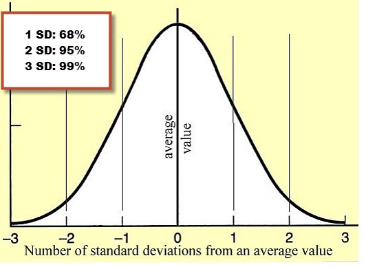
Standard deviation: normal bell curve
Calculations for 1 month and 1 standard deviation
Since very few of us trade 1-year options, these implied volatility stats must be customized to our shorter-term periods. It’s not necessary to remember this math but you’re getting it anyway…
For a 30-day option and 1 standard deviation, we multiply the implied volatility stat by the square root of 30/365:
$30 x 20% x .286 = $1.72
This means that based on current option pricing, we would expect this stock to trade between $28.28 and $31.72 68% of the time during the next 30 days (I’m beginning to give myself a headache!).
Summary
Implied volatility is more important to short-term option sellers than is historical volatility. It demonstrates market sentiment about future price movement although does not define direction. We can use it to determine price probability and therefore risk parameters that will allow us to decide if a trade is consistent with our personal risk-tolerance and monthly goals. A quick, user-friendly way to estimate implied volatility is to look at the returns on an option. For example, if a 1-month at-the-money strike generates more than 6%, we are dealing with a high-implied volatility trade. This may be appropriate for some but not for others.
Next live seminar:
February 6, 2015
The World Money Show Orlando, February 6, 2015 at The Gaylord Palms
Friday February 6th
4PM – 6PM
(I am an invited speaker. The Money Show is charging an admission fee to attend).
The Federal Reserve’s mid-week commentary that the US economy was expanding at a solid pace and generating strong job growth generated market concern that interest rates may be raised sooner than anticipated. Lower interest rates are favorable for the stock market. There was also concern of declining oil prices which picked up on Friday resulting in a late-day selloff. This shows how unpredictable our markets can be. This week’s mixed reports:
-
According to the Commerce Department, gross domestic product (GDP) in the 4th quarter declined to 2.6%, below the 3.1% projected by analysts
-
For the year 2014 our economy expanded by 2.5%, above the recent trend of 2%
-
Durable goods orders fell by7 3.4% in December as analysts were expecting a rise of 0.5%. This was the 4th decline in 5 months
-
New home sales in December rose to an impressive annual rate of 481,000, well above the 450,000 anticipated
-
Year-over-year new home sales rose by 8.8%
-
The median price for new homes sold in December rose from $291,600 (in November) to $298,100. This represented an increase of $22,600 year-over-year
-
The Conference Board’s Consumer Confidence Index in January increased to an impressive 102.9 well above the 95.0 expected. This represents the highest level since August, 2007
For the week, the S&P 500 fell by 2.8%.
Summary
IBD: Uptrend under pressure
GMI: 3/6- Buy signal since market close of January 23, 2015
BCI: Cautiously bullish but favoring in-the-money strikes 2-to-1 for new positions as a hedge against recent market volatility
Wishing you the best in investing,
Alan (alan@thebluecollarinvestor.com)
Premium Members,
This week’s Weekly Stock Screen And Watch List has been uploaded to The Blue Collar Investor premium member site and is available for download in the “Reports” section. Look for the report dated 01/30/15.
Also, be sure to check out the latest BCI Training Videos and “Ask Alan” segments. You can view them at The Blue Collar YouTube Channel. For your convenience, the link to the BCI YouTube Channel is:
http://www.youtube.com/user/BlueCollarInvestor
Since we are in Earnings Season, be sure to read Alan’s article, “Constructing Your Covered Call Portfolio During Earnings Season”. You can access it at:
https://www.thebluecollarinvestor.com/constructing-your-covered-call-portfolio-during-earnings-season/
Best,
Barry and The BCI Team
Alan,
I follow your articles on my Netvibes aggregator. This is an especially interesting and important one. I agree with your basic viewpoint that implied volatility (IV) is more important to covered calls investors, but I’d like some discussion of the use of historical volatility (HV). I prefer to sell options where IV>20, but I also look at the 90-day HV. I’m especially fond of selling options when the IV is significantly greater than the HV(90) and there is no earnings report before the expiration date. Do you consider HV at all in your analysis, or do you consider it totally irrelevant?
Jeff
Jeff,
I definitely would NOT use the word “irrelevant” as it relates to historical volatility. As a matter of fact, we use “beta” stats in our Premium Stock Reports. As you know, these are historical measurements of a security’s volatility as it relates to the overall market, usually the S&P 500.
The reason I put more significance into IV stats is because of the short-term nature of the option-selling strategies we use (one month or less in most cases). Market opinion is factored in with IV. Now, if I were looking for a stock for a long-term buy-and-hold portfolio, HV would be more significant to me.
I consider IV a primary factor in my short-term option decisions and HV, a secondary factor. For example, if I am deciding between 2 securities with similar primary features and returning similar initial returns, I may use beta to “break the tie” Low-beta stocks tend to out-perform in bear markets and high-beta stocks tend to out-perform in bull markets…tie broken.
I’m sure you have specific reasons why you set the parameters you mentioned and if they have met the test of time, there is no reason not to stay with them.
Alan
I understand the concept of IV and the standard deviation and the probability of expiration of options. However, I have difficulty in using this to select the strike price, which is the whole essence of this exercise.
The conundrum is that if you go out to 1 SD, and select options with probability of expiring at 61.8% than the premium that one would receive would be far lower than if one selects an ATM strike price. The problem is that the latter strike would most certainly require adjustment while that at 1 SD has lower premium but higher probability.
How can I determine a strike price that is somewhere in between these two scenario, giving me value of the strike that will maximise the returns.
many thanks
sean
Sean,
Strike price selection is one of the three skill sets required to become an elite options-seller. Stock selection and position management are the other two. The purpose of this article was to show the role of implied volatility in our option premiums and the risk incurred. Once these concepts are understood, it will facilitate strike price selection based on several factors:
1- Overall market assessment
2- Chart technicals
3- Personal risk-tolerance
4- Initial goals/time frame (mine is 2-4%/month in normal market conditions)
There is no one formula that is appropriate for every investor but by using the principles in this article and others discussed in my books/DVDs we can all develop a formula that meets our needs and trading styles.
For example, an investor with a higher risk tolerance, in a bull market environment, with strong chart technicals may use a higher IV option and shoot for a 5-7%, 1-month return for a near-the-money strike. The “moneyness” of the strike also needs to be selected. ITM strikes are more conservative than OTM strikes.
In the Complete Encyclopedia…this topic is discussed in detail in pages 108 – 124.
Alan
Alan, In your recent reply to me you had said of your “Mixing of strikes” rule that you always use, but am wondering if we can still be successful with selling covered calls if we don’t want to do any of the mixing of strikes for the same stock, or others each month, even though you do?(it just seems to me rather complex and needing more time involvement.)?
2. I need to go over some price performance issues I have, and have told you that I will also use the ‘RS line’ for even greater confirmation.
Now if I see this RS line showing some underperformance(maybe in the form of a support level break,etc) and the stock price confirms this also by a break of support level,etc too, then wouldn’t it be better for me to close out this stock rather than wait for it to drop to the 20%/10% level to then decide what to do?
3. For the above, I don’t quite understand why to first wait for a stock to drop up to say 10- 15% or so, to then reach the 20%/10% levels before deciding that it would be best to close the position, when it could have been done earlier with the ‘RS line’ indicator of underperformance?
4. And one other thing,- in case of my concern for a stock to drop rapidly, then is it alright for me to set-up an order in advance to close out my entire position once the price goes below a certain price? (e.g. the recent price low is at $46, so put in a sell order for at $45.99 or lower – but as long as the call option is to always be bought back first?- hope a broker could do this?)
I quite like this certain indicator, have used it a while and am getting better results than I used to and so that is why I continue to. Thanks for your help with this.
Adrian,
I have found that strike selection is one of the three skills needed to become an elite covered call writer. I believe in taking advantage of every edge possible. You stress technical analysis as I do. If a chart is mixed rather than all bullish and confirming I favor ITM strikes in normal market conditions. If the chart is bullish and confirming, I favor OTM strikes. In strong bull markets I may favor OTM strikes even with a mixed technical picture. It may take a bit more time (not much once you master this approach) but it will pay significant dividends in the long run. You can be successful using only one type of strike but (in my view) not as successful as an option seller who mixes strikes based on the factors we have previously discussed.
If you want to use % of share depreciation to close a position, ask your broker about an “OTO” order (one triggers other). This may meet the needs of your trading style. Just make sure you don’t find yourself in a naked options scenario. Another possibility, is to ask for an alert sent to you when the stock price reaches a certain price point and then take action.
Alan
Dear Alan,
I received your book about exit strategy and I deeply appreciated!
I have been invest whit covered option for my first month and I generate a monthly return of 1.1%. I’m happy because I’m a beginner, but at the same time I would like to improve to a better level of 2% or 3% monthly basis. Did you have any recommendation or advice about where I need to focus more to get better result? Strike prices, trend, exit strategy, volatility…
I know is generic, but i guess you can give me a Idea.
Again Alan, thanks so much for the great job you have done for the investors community!
Best Regards
Stefano
Hong Kong
Stefano,
You’re doing great so far. You will only get better. The best way for most investors to achieve the highest returns is to continue the education process and gain confidence through experience. Take your time and stay conservative. Give yourself several months to reach a higher comfort level. Increased returns will be a result of your due-diligence and education.
Keep up the good work (did I say stay conservative especially at the beginning!).
Alan
Hi Alan
looking at the option chains and noticed with almost 3 weeks until feb20 expiration the in the money strikes had very little if any time value! otm had some decent premiums this makes me think if you sell an itm call and there is a drop in the stock price the option premium could drop dollar for dollar ( a nice way to profit and buy back the call) the fluctuation of the stocks is a real
powerful ingredient to making money!
enjoying the book
thanks Bruce
Hi Bruce,
You commented on two important points:
1- The deeper in (or out for that matter) -the-money we go, the lower the time value component of the option premium. At-the-money strikes generate the highest initial returns but that does not necessarily mean we should always use ATM strikes.
2- The deeper ITM the strike the higher the delta. This means the option value will change close to dollar-for-dollar with the underlying security.
Glad you like the book.
Alan
Alan, if I can confirm something first from your answers before dropping more questions to you.
For the answers to my No’s ‘2 & 3’ above, the picture that I am imagining is that when I incorporate and use the RS line in my analysis, that I should treat it just like the MACD, and Stochastics indicators, whereby they can all set the scene for if the technicals on a whole are to be viewed as positive or mixed.
So if the RS line(I will also use) breaks it’s uptrend-line, then you are saying that because of this, it would bring in a more mixed technical view to the chart?(rather than a positive one – from still being in an uptrend)?,- is this how I should analyse things?
There’s 2 questions out of my curiosity on trading around support levels:- 2. Do you when you want to rolldown or CDMP on any of your stocks try have a trade filter for this,- like sell only if price has dropped below the lowest price at a recent support level, etc?
3. Are you more likely to rolldown earlier than the 20%/10% values, if the percentage value of this stock option is starting to get close these 20%/10% levels, and the stock price goes and breaks a support level, or wouldn’t this affect your decision? (I’m sort of thinking here that there is an added probability of further price declines)?
4. Also if the earliest time I can put on a trade (or close one out) is 11am, then is it possible to instruct the online broker to put in either a limit-order or market-order trade but only from 11am, if I was putting this order on the night before from overseas?
I am living outside the USA and like a lot of other people would just have to adjust to the different time schedule which I guess could be quite challenging, when and if I start trading. Thank you very much.
Adrian,
I do view technical analysis as an art as much as a science. Although we would like TA to give us precise answers, it does not. However, it is a huge asset in our analysis, one that we cannot do without, in my view. If the RS line shows a breach where the stock is under-performing the overall market, I would categorize the technicals as mixed. This will influence our investment decisions as far as strike selection and position management. Keep in mind that overall market assessment plays a major role as well. For example, if technicals are mixed but we are in a raging bull market, I will usually still favor OTM strikes.
Check with your broker on the timing of your trades and if they cannot accommodate you, consider using buy-write combination forms to enter trades from outside the US.
Alan
Premium members:
This week’s 6-page report of top-performing ETFs and analysis of ALL Select Sector Components has been uploaded to your premium site. The report also lists Top-performing ETFs with Weekly options.
For your convenience, here is the link to login to the premium site:
https://www.thebluecollarinvestor.com/member/login.php
NOT A PREMIUM MEMBER? Check out this link:
https://www.thebluecollarinvestor.com/membership.shtml
Alan and the BCI team
Hi Alan, just out of curiosity;
Have you tried selling naked puts and covered calls together, on the same stock?
Say I split 50-50 allocated money for this trade between put and covered calls.
The reason is that if the stock quickly runs up, I can buy back for much cheaper the puts and thus realize a profit on this part and if price persist higher the stock will be called away with another part of a profit.
If the stock goes hard down, I can buy back the calls for cheap and perhaps have an opportunity for a double hit if it bounces back.
If the stock doesn’t come back and I get put the stock, this way I’ll have purchased the stock for even less then the original purchase to cover the call, thus lowering my average stock purchase base.
If you have a minute, can you comment on this, what you think?
Thanks,
—
Ryszard
Ryszard,
Nothing at all wrong with mixing two great strategies. I still give a slight edge to covered call writing in normal and bull market environments and tend to favor put-selling in a bearish or volatile market environment. That said, both strategies can be extremely effective in most market conditions.
You can also mix strategies using the PCP Strategy discussed in Chapter 16 of my latest book.
Alan